


Since I've been dealing a lot recently with concepts like "Embedding," "User Behavior Prediction," and "Marketing," I happened to read a paper that combines all three: CXSimulator: A User Behavior Simulation using LLM Embeddings for Web-Marketing Campaign Assessment. The method in the paper isn't hard to understand, but it has what I consider a lot of "clever little tricks." It once again gave me that long-lost thrill of seeing smart algorithms cleverly applied to specific constraints. So today, I'm sharing the method from this paper.
Background
For many e-commerce or internet platforms, new products, new pages, and various marketing campaigns are launched almost every day. These changes affect the user's subsequent browsing paths and ultimate conversion rates. The most common and direct validation method right now is A/B testing: launching two versions of a page and showing them to random users to observe target metrics. The results of a proper A/B test are, of course, the most reliable, but the problem is also obvious: every experiment consumes real traffic and development costs. So, is it possible to simulate user behavior and predict in advance whether a change is worth rolling out before the campaign actually goes live? This is undoubtedly a massive pain point.
And this paper's solution is to use behavioral semantics to predict state transitions, and then simulate user behavior through Markov chains.
Algorithm Introduction
First, let me attach a figure from the original paper. This image actually directly shows the complete architecture:
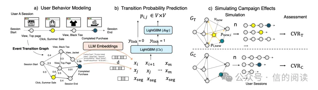
But it's pretty hard to understand just by looking at the picture. So next, I'll follow the logical order in the diagram and explain exactly what this algorithm does in the most straightforward way possible.
Step 1: Understanding the Data
First, we need to get a general understanding of our data. User data on a page can roughly be described as a series of sequential behaviors. I'll just give one example here:
Behavior sequence starts > Home Page > Product Details > Checkout > Behavior sequence ends
The example here is super simple: a user enters the website's home page, then goes to the product page, and then proceeds to the checkout page. The real process involves all sorts of behaviors. For example, very short sequences where they only look at the home page. Or back-and-forth behaviors, bouncing between two pages. Or very long, non-repeating exploratory behaviors, and so on. But every user's browsing history is basically a series of action records like this.

Step 2: Calculating the State Transition Graph
Once we have this kind of dataset, the first thing we need to do is build a state transition graph, which is exactly the graph in the paper:
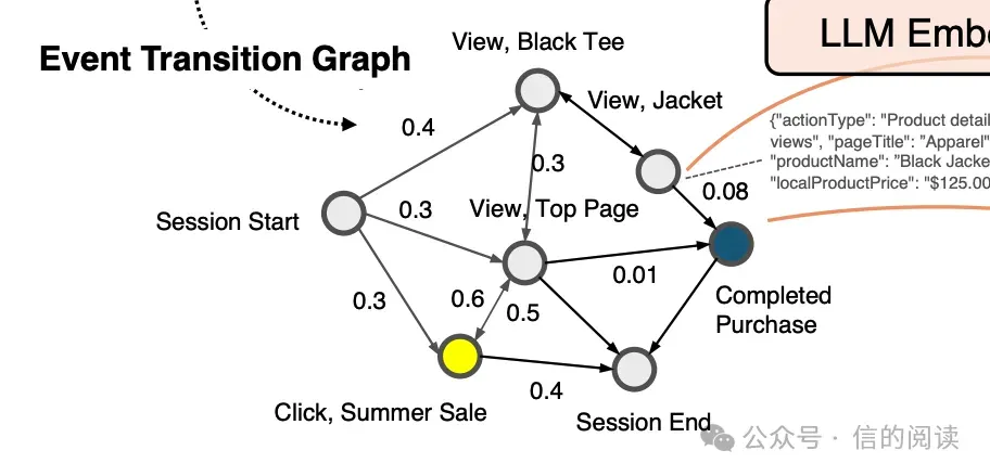
Each node in the graph represents a specific behavior from the previous example, like entering the home page or entering the product page. Of course, in real data, every specific product would also have its own node.
Then, based on all the data, we can calculate which other nodes each node can connect to, and calculate the transition probabilities. For instance, let's say we observe the following behaviors and counts after the behavior "Viewing Black Tee":
- 60 times > Add to Cart
- 25 times > View other products
- 10 times > Checkout
- 5 times > session_end
Then we can calculate the probability of each subsequent behavior after "Viewing Black Tee":
- Viewing Black Tee > Add to Cart: 60 / 100 = 0.60
- Viewing Black Tee > View other products: 25 / 100 = 0.25
- Viewing Black Tee > Checkout: 10 / 100 = 0.10
- Viewing Black Tee > session_end: 5 / 100 = 0.05
It's worth noting that the probability here depends only on the current node, and has absolutely nothing to do with what behaviors were experienced previously. And this is exactly the assumption of a First-order Markov Chain! Therefore, the entire user behavior graph is essentially a state transition graph. This is also one of the limitations of this algorithm, because a user's next action often depends on more than just the "one" preceding action, but rather a culmination of a series of actions. However, to simplify calculations, making this kind of trade-off is something we frequently do in practical applications.
The resulting transition probability matrix looks like:
| Transition | Probability |
|---|---|
| A > B | 0.62 |
| A > C | 0 |
| A > D | 0 |
| A > E | 0 |
| ... | ... |
| B > C | 0.31 |
| ... | ... |
Step 3: Training the State Transition Prediction Model
This is the most important step of the whole algorithm. It's exactly the approach taken in this step that opens up the possibility of introducing new "marketing campaign" nodes later on.
Our goal in this step is to train a model that can predict the transition probability from one node to another. So, we face two questions: how do we choose the model's input and output?
Model Input
If we directly use node IDs or other discrete encodings (like One-hot) to represent nodes, the model could indeed learn the relationships between nodes that already exist in historical data. But don't forget, the goal of this paper is to predict new marketing campaigns that might appear in the future and have never appeared in historical data. If we use this kind of discrete representation, the model won't be able to handle new nodes because they don't have a corresponding ID. Therefore, nodes must be represented as continuous vectors (Embeddings) with semantic information, so the model can generalize to unknown nodes.
Naturally, we can use an Embedding model here to convert the text description of each node into vector data as the feature information for that node. I think this step is the most ingenious design in the entire paper, and the most critical link between historical data and future unknown nodes. So, the data on the input side of the model consists of ordered node pairs, like:
- (Home Page, Product Page)
- (Product Page, Black Tee)
- (Black Tee, Checkout Page)
And each node is no longer the text itself, but a vector representing its meaning.
Model Output and the Sparsity Problem
The input side is sorted out, but what about our output? The output seems simple enough, because we've already calculated the transition probability for every connected pair, so we just need a regression model to predict the probability for each connection. But think about it carefully, and you'll quickly spot a problem. Let's use a very intuitive example:
Assume the entire graph has 1000 nodes. Theoretically, there are 1000 x 1000 = 1,000,000 possible node combinations. But the actual existing edges might only be 8000. So the training data becomes extremely sparse: the vast majority of the samples have a label of 0.
Anyone who has trained models knows that if you directly train a regression model on such extremely sparse data, the easiest strategy for it to learn is "predict everything as 0." Even though the final loss might not be high (and it will likely be very low, because the model can achieve a low loss just by always predicting 0), the model pretty much loses its ability to predict real connections.
Two-Stage Modeling
So, the paper's actual approach is to do this in two steps. First step: train a classifier model to predict whether there is a connection between the two input nodes. Second step: train a regression model to predict the transition probability between the two nodes. During the prediction phase, only the node pairs that the classifier determines to have a connection will be passed on to the regression model to predict their transition probabilities. The paper uses LightGBM for both models, which is essentially a Gradient Boosting Decision Tree (GBDT). It can act as both a classifier and a regressor.
Step 4: Simulation
Now we have all the model resources needed to simulate a new marketing campaign. If at this point we have a new marketing activity, for example, adding a "Tea Product Click Discount" page, our simulation process goes like this:
Predicting Connections for the New Node
First, using the exact same Embedding model as in training, we convert the page information of "Tea Product Click Discount" into a vector in the same dimensional space.
Then, we take the marketing page's information and all the existing node information, and input them sequentially and individually into our classification model and regression model for prediction. For example:
Input 1: [View Home Page, Tea Product Click Discount] > Classifier > Connection Exists (0.91) > Regressor > 0.35
Input 2: [View Home Page, Tea Product Click Discount] > Classifier > Connection Exists (0.97) > Regressor > 0.68
Note that our inputs need to be bidirectional. That means we have to run predictions for both [View Home Page, Tea Product Click Discount] and [Tea Product Click Discount, View Home Page] to get their transition probabilities. For those where the classifier predicts no connection, we don't need to run the regression prediction, and we don't need to add a corresponding connection in the graph either.
Normalizing the New Node's Outgoing Probabilities
Once all the predictions are complete, we need to update a control group graph. Since we just added the new "Tea Product Click Discount" node, and we've predicted its probabilities to all other outputs, here's an example:
- Tea Product Click Discount > View Longjing Product: 0.40
- Tea Product Click Discount > Add to Cart: 0.20
- Tea Product Click Discount > Checkout: 0.10
We notice that the sum of all predicted probabilities doesn't equal 1, so we just need to normalize them. Sum of predicted probabilities: 0.40 + 0.20 + 0.10 = 0.70. So we normalize:
- Tea Product Click Discount > View Longjing Product: 0.40 / 0.70 = 57%
- Tea Product Click Discount > Add to Cart: 0.20 / 0.70 = 29%
- Tea Product Click Discount > Checkout: 0.10 / 0.70 = 14%
Ultimately, the sum of these three outgoing edge probabilities becomes 1 again.
Updating Existing Nodes
The probabilities for other existing nodes need to be updated as well. Let's assume the original "View Green Tea Product" node had three outgoing edges:
- View Green Tea Product > Add to Cart: 60%
- View Green Tea Product > View other products: 30%
- View Green Tea Product > session_end: 10%
Now our regression model predicts a newly added probability edge from "View Green Tea Product" to "Tea Product Click Discount": 0.25
We can't just add 0.25 directly to the existing probabilities, because then the sum would definitely exceed 1: it would become 1.25. So, we use 1.25 as the total sum to normalize again:
- View Green Tea Product > Add to Cart: 0.60 / 1.25 = 48%
- View Green Tea Product > View other products: 0.30 / 1.25 = 24%
- View Green Tea Product > session_end: 0.10 / 1.25 = 8%
- View Green Tea Product > Tea Product Click Discount: 0.25 / 1.25 = 20%
Through this, we've used the model to add a previously non-existent node into the original First-order Markov Chain graph, and rationalized all the transition probabilities.
Running the Simulation
What happens next is super simple. We randomly sample N user paths through the original graph and calculate a specific conversion rate. For instance, out of N paths, if M paths eventually lead to payment, the conversion rate is M/N. Then, we run a random simulation of N user paths in the new graph that includes the marketing campaign. Assuming we collect K paths that lead to payment, the conversion rate is K/N. And the final impact of our marketing campaign is simply the difference between K/N and M/N.
Limitations and Broader Impact
Of course, the method proposed in this paper has plenty of limitations. Can semantic embedding truly represent the meaning of a user's behavioral space? Does the First-order Markov Chain assumption really hold up? The model assumes by default that a new marketing activity can establish connections with all historical nodes, whereas in reality, a marketing page usually only appears in a few fixed locations. These are all assumptions that need validating.
But I think none of these limitations negate the inspirational value of this paper. What really made my eyes light up was that it offers a completely fresh perspective: abstracting user behavior into a state transition graph, using an Embedding model to provide semantic generalization capabilities, and then completing offline simulation (as opposed to online A/B testing) through probability models and Markov chains. This combination of "Embedding + Graph + Probability Model + Simulation" isn't just applicable to marketing; it provides a highly referenceable solution framework for a lot of user behavior simulations, strategy evaluations, and even Agent simulation problems.